ML for Digital Humanities #02 — From a Single Global Line to Group-Specific Relationships

In the previous post, we discovered something interesting: using only rim diameter, we were able to approximate vessel height with a certain degree of precision. But we also realized something less positive. More than half of the variability remained unexplained by the data. This raised a natural question: could we perhaps be oversimplifying the problem?

Interactive Notebook Available:

All the code and analysis in this article is also available as a Jupyter Notebook. Click the button above to run it interactively in Google Colab (no installation needed).

If rim diameter alone is not enough to build a model capable of explaining the variability of the pieces, the most likely explanation is that explanatory elements are missing — in other words, that there are variables escaping us. Let us move to a very distant but highly didactic example. Imagine that we want to estimate the weight of an animal solely from its length. If we mix dogs, cats, horses, and rabbits into a single graph, we will obtain a general relationship: the greater the length, the greater the weight. But that line will be very clumsy, because a dog and a rabbit may have similar lengths and very different weights.

Length matters, yes, but it does not mean the same thing across all groups. Within dogs, the relationship between length and weight may be fairly coherent. Within cats as well. But if we mix all animals together as though they were a single biological reality, the global regression line begins to lose meaning.

This is why the question changes. It is no longer simply:

“Can we estimate weight from length?”

but rather:

“Can we estimate it better if we also know what type of animal we are observing?”

Something similar may be happening with archaeological ceramics. Our model explains only part of the variability of the dataset, probably because we are using a single variable. But what would happen if we introduced another variable into the analysis — the one defining the type of ceramic object, the typology: jar, bowl…? Would estimation improve for each typological category? Let us see.

With this approach, we could draw two very different scenarios. On the one hand, we could use the form variable to separate the dataset and perform a Linear Regression for each subset, thereby avoiding distractions caused by other ceramic types. On the other hand, we could build a multiple linear regression by combining this new variable with the one we already had. Let us begin with the first case.

Linear Regression by Category

We will start from the same base file used at the beginning. The variable we will add to our analysis is the form type: vessel_form. We begin by loading the dataset, cleaning the relevant columns, and filtering to the five most represented typologies:

import pandas as pd
import numpy as np
import matplotlib.pyplot as plt

from sklearn.linear_model import LinearRegression
from sklearn.metrics import r2_score, mean_squared_error
from sklearn.model_selection import train_test_split
from sklearn.compose import ColumnTransformer
from sklearn.preprocessing import OneHotEncoder
from sklearn.pipeline import Pipeline

# Load data
file_path = "/content/MimPIDD_Public_March_2020.xlsx"
df = pd.read_excel(file_path, sheet_name="MimPIDD_Public_Images")

# Column names
x_col = "rim_diam"
y_col = "height"
cat_col = "vessel_form"

# Clean: convert to numeric, drop missing values
data = df[[x_col, y_col, cat_col]].copy()
data[x_col] = pd.to_numeric(data[x_col], errors="coerce")
data[y_col] = pd.to_numeric(data[y_col], errors="coerce")
data = data.dropna(subset=[x_col, y_col, cat_col])

# Keep only the five most represented typologies
selected_forms = ["Bowl", "Flare rim bowl", "Flower Pot Bowl", "Seed Jar", "Jar"]
data = data[data[cat_col].isin(selected_forms)]

Let us first examine, in a simple table, the existing typologies and the number of pieces in each one:

Typology	Number of pieces
Bowl	1852
Flare rim bowl	114
Jar	48
Seed Jar	30
Flower Pot Bowl	28
Effigy	8
Bowl, Miniature	5
Other	4
Bowl, Flare rim bowl	3
Pitcher	3
Ladle	2
Bowl, Other	2
Bowl, Other, Plate	1
Effigy, Jar	1
Ladle, Other	1

It is important to clarify that this first table shows the original counts from the database. However, not all pieces contain valid values for rim_diam and height. After converting both variables to numeric format, removing incomplete records, and keeping only the selected categories, the effective number of observations used in the analysis is reduced.

As can be observed, there is a huge imbalance. Some categories contain only 1, 2, or 3 pieces, a quantity far too low to extract stable conclusions. In order to produce minimally interpretable results, we will retain only the most numerous typologies: Bowl, Flare rim bowl, Flower Pot Bowl, Seed Jar, and Jar. These are the typologies on which we will perform independent linear regressions, later representing them together in a single graph.

plt.figure(figsize=(11, 7), dpi=120)

colors = plt.cm.tab10.colors

for i, form in enumerate(selected_forms):
    subset = data[data[cat_col] == form].copy()

    if len(subset) < 2:
        continue

    X = subset[[x_col]]
    y = subset[y_col]

    model = LinearRegression()
    model.fit(X, y)

    y_pred = model.predict(X)
    r2 = r2_score(y, y_pred)

    color = colors[i % len(colors)]

    plt.scatter(
        subset[x_col], subset[y_col],
        alpha=0.28, s=28, color=color,
        edgecolor="white", linewidth=0.4,
        label=f"{form} (data)"
    )

    x_range = np.linspace(
        subset[x_col].min(), subset[x_col].max(), 200
    ).reshape(-1, 1)

    plt.plot(
        x_range, model.predict(x_range),
        linewidth=2.6, color=color,
        label=f"{form} trend | R²={r2:.2f}"
    )

plt.xlabel("Rim diameter (cm)", fontsize=12)
plt.ylabel("Height (cm)", fontsize=12)
plt.title("Linear Regression by Vessel Form\nRim diameter → Height",
          fontsize=15, weight="bold", pad=14)
plt.grid(True, alpha=0.18)
plt.gca().spines["top"].set_visible(False)
plt.gca().spines["right"].set_visible(False)
plt.legend(bbox_to_anchor=(1.02, 1), loc="upper left", frameon=False, fontsize=9)
plt.tight_layout()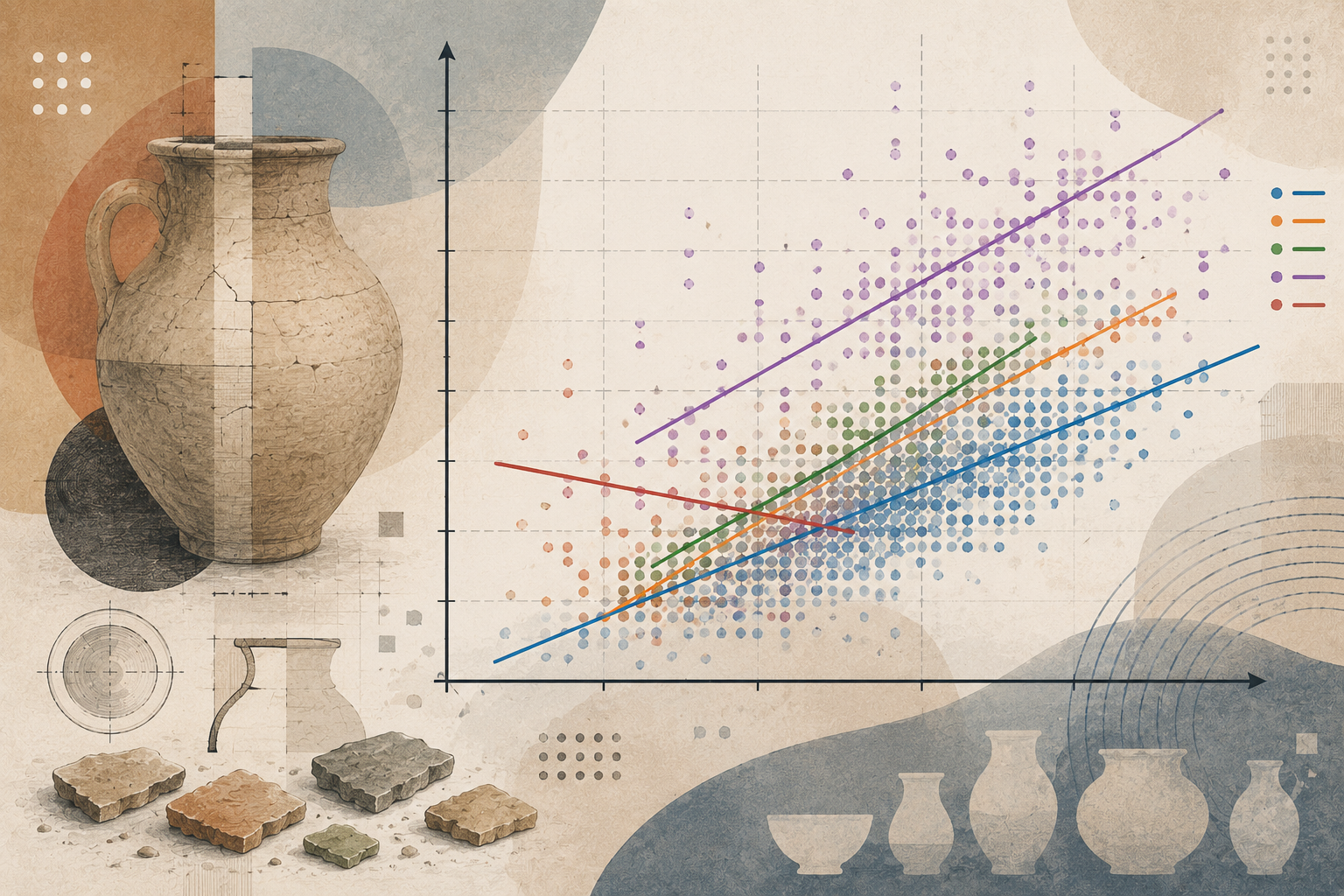
plt.show()

The result obtained was one regression line for each ceramic typology derived from the data. In general, except for the regression corresponding to Seed Jar, the others show a positive relationship: as rim diameter increases, height also tends to increase. This case — Seed Jar — is not entirely surprising, since, as previously mentioned, it is extremely difficult to model from so few pieces.

Having reached this point, let us analyze the results using two measures: the coefficient of determination (R²) and the RMSE (Root Mean Squared Error). The following table summarizes the behavior of each category represented independently using the previously cleaned data:

Vessel form	Samples	R²	RMSE
Bowl	1435	0.572	1.864
Flare rim bowl	98	0.447	1.710
Jar	16	0.394	5.393
Flower Pot Bowl	27	0.376	2.115
Seed Jar	16	-0.854	2.881

results = []

for vessel in selected_forms:
    subset = data[data[cat_col] == vessel].copy()

    if len(subset) < 10:
        continue

    X = subset[[x_col]]
    y = subset[y_col]

    X_train, X_test, y_train, y_test = train_test_split(
        X, y, test_size=0.25, random_state=42
    )

    model = LinearRegression()
    model.fit(X_train, y_train)
    y_pred = model.predict(X_test)

    results.append({
        "Vessel form": vessel,
        "Samples": len(subset),
        "R²": round(r2_score(y_test, y_pred), 3),
        "RMSE": round(mean_squared_error(y_test, y_pred) ** 0.5, 3)
    })

results_df = pd.DataFrame(results).sort_values(by="R²", ascending=False)
print(results_df)

For each of these categories, an independent linear regression was trained. In every case, the model was trained using 75% of the available data for that typology and evaluated on the remaining 25%. This allows us to observe not only how well the line fits known data, but also how it behaves on data not used during training.

These data provide a great deal of information, especially when compared both against each other and against the exercise performed in the first publication. In the previous global model, the relationship between rim diameter and height explained approximately 42% of the variability of the complete dataset. When analyzing only bowls, that relationship reaches an R² of 57%. This does not simply mean that the model “improves,” but rather that within this category the geometric relationship between both variables appears more stable.

This is particularly interesting because Bowl is not only the category with the highest number of samples (1435), but also the most visually heterogeneous one. Despite this, the model displays greater explanatory power when this category is analyzed in isolation. This suggests that part of the “noise” present in the initial model did not necessarily come from the internal variability of bowls, but rather from the mixture of different ceramic forms probably governed by distinct geometric proportions.

However, not all categories behave in the same way. Flare rim bowl, despite having far fewer samples, still maintains a relatively consistent behavior, achieving an R² of 0.447 and an RMSE even lower than that of Bowl. This could indicate greater formal homogeneity within this specific category.

By contrast, categories such as Jar or Flower Pot Bowl produce considerably more modest results. Here we must be cautious. A lower R² does not automatically imply that the relationship between diameter and height does not exist, but rather that other factors probably intervene which the model is not yet considering.

In archaeology, this has particular importance. The proportions of a piece do not depend solely on an abstract geometric logic. Functional considerations, craft traditions, regional differences, chronology, and even possible inconsistencies in typological classification also play a role.

The case of Seed Jar is particularly revealing. When evaluating the model on data not used during training, it obtains a negative R² (-0.854). This means that, for that testing subset, the regression predicts worse than a naïve estimation based simply on the mean. The result should not be interpreted as a definitive truth about Seed Jars, but rather as a signal of instability: with only 16 valid examples, small variations in the training-test split can greatly alter the outcome.

Multiple Linear Regression

As previously indicated, the second scenario consisted of incorporating the vessel_form variable into a single model alongside rim diameter. In this case, we no longer train an independent regression for each typology, but rather a single model simultaneously using a numerical variable (rim_diam) and a categorical variable (vessel_form) to estimate vessel height.

In order to include the typological variable in the model, it was transformed using One-Hot Encoding. In other words, each vessel_form category was converted into a binary variable indicating whether a piece belongs to a specific form or not. In this way, the linear regression can use typological information in addition to rim diameter.

X = data[[x_col, cat_col]]
y = data[y_col]

X_train, X_test, y_train, y_test = train_test_split(
    X, y, test_size=0.25, random_state=42
)

preprocessor = ColumnTransformer(
    transformers=[
        ("cat", OneHotEncoder(drop="first", handle_unknown="ignore"), [cat_col]),
        ("num", "passthrough", [x_col])
    ]
)

multiple_model = Pipeline(
    steps=[
        ("preprocessor", preprocessor),
        ("model", LinearRegression())
    ]
)

multiple_model.fit(X_train, y_train)
y_pred_multiple = multiple_model.predict(X_test)

r2_multiple = r2_score(y_test, y_pred_multiple)
rmse_multiple = mean_squared_error(y_test, y_pred_multiple) ** 0.5

print(f"R²:   {r2_multiple:.3f}")
print(f"RMSE: {rmse_multiple:.3f}")

The model was trained using 75% of the data and evaluated on the remaining 25%. The resulting performance was an R² of 0.641 and an RMSE of 1.978. This indicates that, by incorporating ceramic form, the model is capable of explaining a larger portion of the variability in height than the initial model based solely on rim diameter.

However, this result must be interpreted carefully. Multiple linear regression improves overall predictive capability, but it does not replace category-based analysis. Both approaches answer different questions.

Multiple regression answers a predictive question:

“Can we estimate vessel height better if we simultaneously use rim diameter and typology?”

The answer appears to be yes. The vessel_form variable provides relevant information and improves model performance.

By contrast, independent regressions by category answer a more interpretative question:

“Does the relationship between diameter and height behave the same way within each ceramic form?”

And here the answer is more complex. Some forms, such as Bowl or Flare rim bowl, display relatively stable relationships. Others, such as Seed Jar or Jar, present more problematic results, probably due to the low number of samples, greater internal variability, or the intervention of factors not yet contemplated by the model.

Therefore, the point is not to decide absolutely which model is “better.” If the objective is to predict the height of new pieces, multiple linear regression appears more appropriate. If the objective is to understand the internal structure of the dataset and observe how different ceramic forms behave, category-based regressions remain indispensable.

This point introduces a crucial methodological issue in machine learning: it is not enough merely to build models; it is also necessary to evaluate the quality, stability, and representativeness of the data with which we work. Furthermore, this breaks a very common intuitive assumption when we begin working with statistical models: the belief that adding more variables or separating categories automatically improves results.

Reality is considerably more complex.

Consequently, what we have attempted in this publication is not so much to build a better model, but rather to delve into the structural complexity hidden within the data, which is far greater than it initially appeared.

And it is precisely here where machine learning ceases to be a simple mathematical tool and begins to become a tool for historical interpretation.

See you in the next one.